Multiplane calibration Grussmayer Lab

Introduction

Multiplane microscopy images several focal planes of a sample simultaneously by splitting the fluorescence emission onto different regions of one or more camera sensors. The raw frames therefore contain a tiled mosaic of planes that are shifted, slightly rotated and scaled with respect to each other, imaged at different effective transmission, and recorded in an order that is not known a priori. mp_proc is our Python toolbox that calibrates a multiplane setup from a bead z-stack and turns the raw acquisitions into ready-to-use, co-registered image stacks.

Calibration

Calibration is performed once per optical configuration on a z-stack of subdiffraction fluorescent beads and is stored as a single calibration file (cal.json) that can be reused for all subsequent measurements taken with the same setup and emission filter.

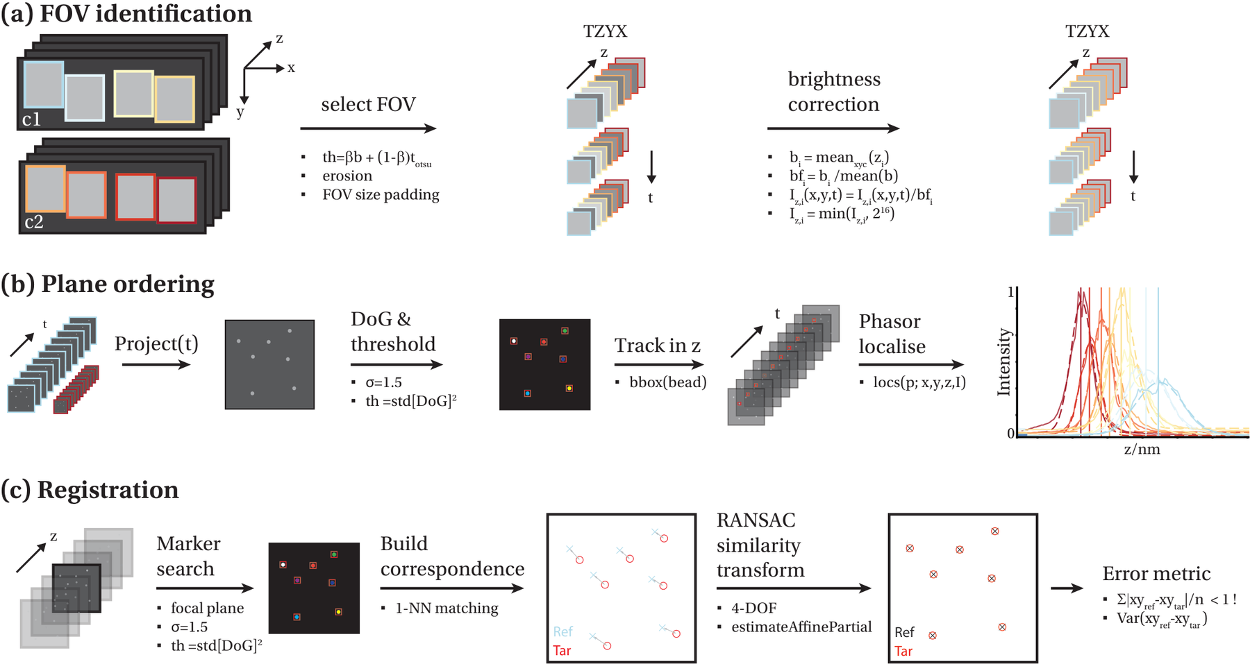
The calibration proceeds in the following steps:

Deskewing - the tilt of the illumination across the sensor is estimated and corrected, so that intensities can be compared between planes.
Plane detection - the individual plane sub-images are located on the sensor by adaptive thresholding, which yields the cropping regions for each plane.
Brightness correction - the relative transmission of the planes is measured and corrected. Because the splitting optics are dispersive, this correction is wavelength dependent and is determined separately for each emission channel.
Axial calibration - fitting a Gaussian to the axial intensity profile of the beads in every plane gives the focal position of that plane. From these positions the interplane distance and, importantly, the physical order of the planes on the sensor are recovered.
Lateral co-registration - the bead positions detected in each plane are matched across planes and an affine transformation (translation, rotation, scaling and shear) is fitted per plane, referenced to a common plane.

Calibration accuracy

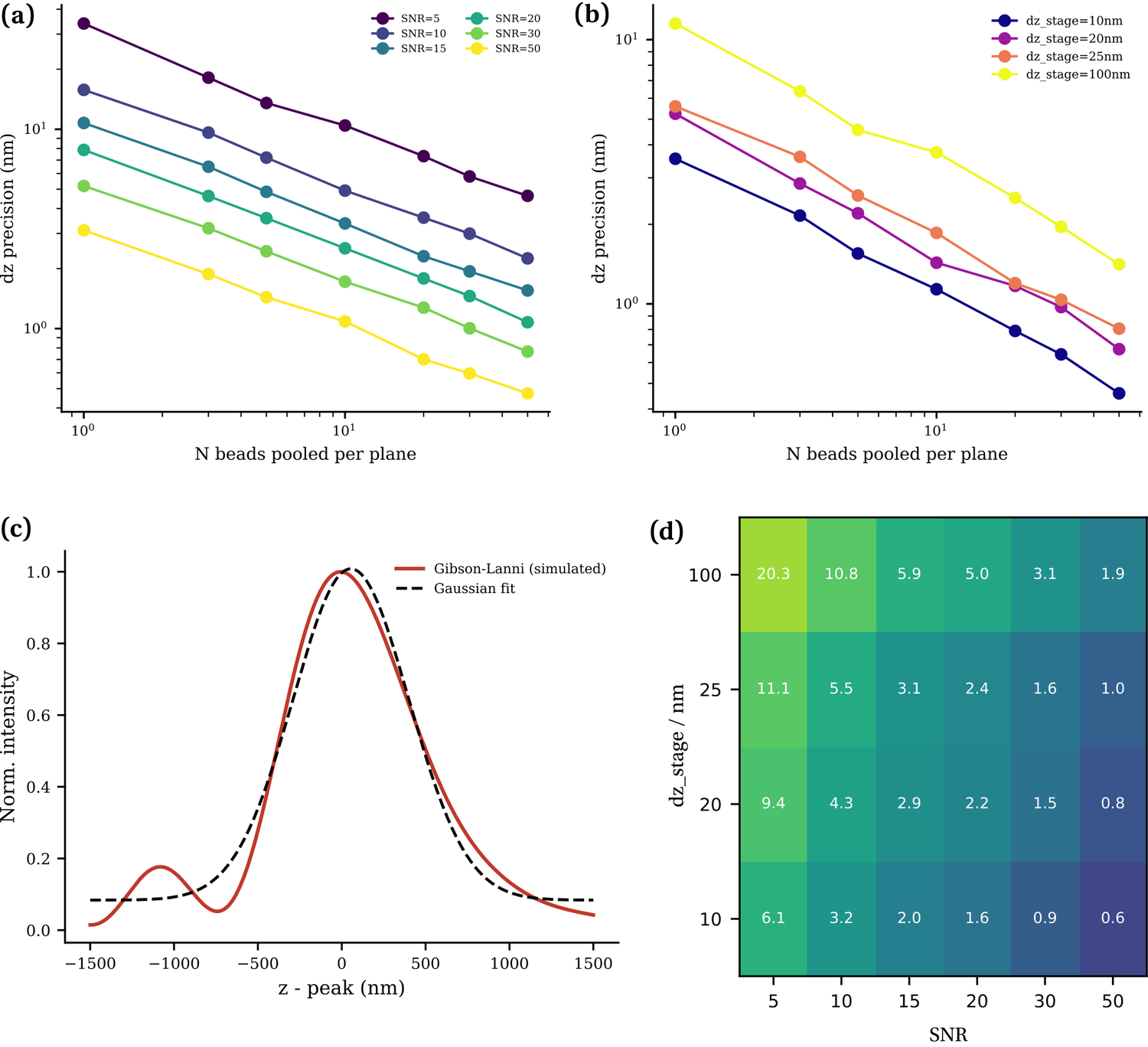
How well the focal position of a plane can be recovered is set by the signal-to-noise ratio of the beads, the stage step of the calibration z-stack and the number of beads that are pooled per plane. Simulations of the axial fit (Gibson-Lanni PSF of a 200 nm bead with spherical aberration and Poisson noise) show that a handful of beads at moderate SNR is already sufficient to reach a few nanometres of precision, well below the interplane distances of several hundred nanometres that are being measured.

Simulated precision of the axial calibration versus SNR, stage step and number of beads — Precision of the axial calibration, from simulation. **(a)** Precision of the fitted focal position against the number of beads pooled per plane, for SNR 5 to 50 at 100 nm stage steps. **(b)** The same for stage steps of 10 to 100 nm at SNR 20 - finer sampling of the calibration stack pays off directly. **(c)** Simulated Gibson-Lanni axial profile against the Gaussian model used in the fit; the model ignores the side lobe but tracks the peak. **(d)** Precision map over SNR and stage step when five beads per plane are pooled, at 561 nm.

Processing

With the calibration file at hand, raw NDTiff or MMStack .tiff files recorded through Micro-Manager are cropped, brightness corrected and warped into a single co-registered stack with the planes sorted by axial position. Data are streamed in batches of frames to keep the memory footprint low, and are written out as TIFF chunks with corrected metadata, ready for further analysis such as SOFI or deconvolution.

Setup parameters - pixel size, number of cameras, number of planes - are set on a MultiplaneProcess instance; calibration and processing are then run from the main_calibration.ipynb and main_processing.ipynb notebooks. The dependencies are listed in requirements.txt and are installed into a conda environment.

Resources

Find the github repository here.